Calculating Power Quantities with Perception Software Calculating Power Quantities with Perception Software | HBM

Calculating Power Quantities with Perception Software

Accurate and highly dynamic power measurements are required for assessing and testing electrical drives in industrial applications, and for hybrid and electric vehicles. This article considers the most important power values, along with some examples. The emphasis is on the use of mathematical formulas in Perception analysis software for power measurements with the GEN2i data acquisition system from HBM.

Introduction

Electrical machines convert electrical energy and mechanical energy. The direction of energy flow is identified by the designation of the mode in which the machine is operating. In motor mode, electrical energy is converted into mechanical energy. In generator mode, the electrical machine is driven and converts mechanical energy into electrical energy. Energy converters are identified by the energy converted per unit of time, rather than simply by the energy that is converted. This value is called instantaneous power, or p(t).

(1.01)

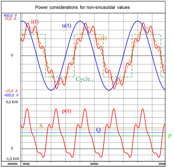
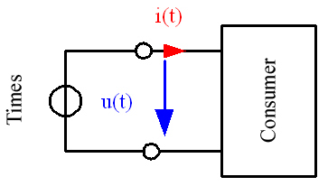
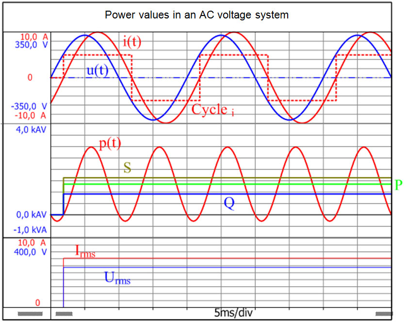
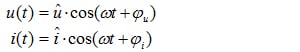
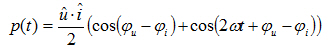
Fig 1.1 shows a two-wire network with an energy source and the corresponding consumer. The applied voltage u(t) and consumer current i(t) can be measured at the measurement points. The instantaneous power is derived from the product of these variables:

(1.02)

The system of consumer count arrows used in Fig. 1.1 shows how the consumer absorbs power when the instantaneous power is positive (p(t) >0). If the instantaneous power is negative (p(t) <0), the consumer feeds power into the source.

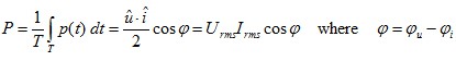
The mean value of the instantaneous power p(t) over the duration of the cycle T is referred to in electrical engineering as the effective power P.


(1.03)

The process for determining active, reactive and apparent power from measured current and voltage curves with Perception is described below.

The implementation of formula (1.03) in Perception software is shown by the example of the extract from the Perception formula database (1.04).
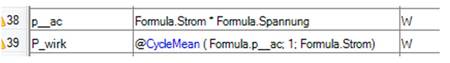

(1.04)

AC Voltage System with Sinusoidal Values

The current that flows in a circuit with linear components and a sinusoidal source voltage in steady state as shown in Fig. 1.1 is also sinusoidal.


(2.01)

The phase shift between current and voltage is derived from the impedance of the consumer. When these conditions are met, instantaneous power is calculated by the following formula:


(2.02)

Fig. 2.1 shows a graph of instantaneous power p(t). This time curve and further power quantities can be calculated with Perception. The results can be verified with the Workbench: AC_power_1.pVWB.

The instantaneous power p(t) oscillates at twice the angular frequency 2ω about its mean value. The mean value is equal to the effective power absorbed by the consumer:(2.03)

The effective power can be calculated in Perception using the mean value of the instantaneous power p(t). The mean value is calculated cyclically based on the duration of the cycle T. The @CycleMean( ) command is used to do this. It is important to detect the correct duration of the cycle. The current curve can be analyzed with the @CycleDetect( ) command for this purpose. This command generates a time function Cycle that returns a 1 in the positive half oscillation and a -1 in the negative half oscillation. This is an easy way to check whether the duration of the cycle has been correctly detected.

In electrical energy, technology the apparent power S serves as a rough guide for designing transmission equipment (cables and transformers, etc.) and for power converters (electrical machines). The effective values of the voltage Urms and current Irms are needed to calculate the apparent power. The following calculations apply to sinusoidal and sinusoidal values:


(2.04)

The apparent power can be calculated from the product of the effective values.

(2.05)

The reactive power Q can be calculated with:

(2.06)


The ratio of the effective power to the apparent power is called the power factor.

(2.07)

The power factor serves as an evaluation of the conversion of energy. Values of the power factor falls within the interval [0,1]. For sinusoidal values, the power factor is λ equal to the shift factor cosφ. If the power factor is λ= 0, no effective power is transferred. The current that is flowing in this state simply loads the lines and other transmission equipment without doing any work. If the power factor λ= 1, only effective power is delivered to the consumer. The load on electrical equipment is as low as possible for the assigned effective power in this state.

Power Considerations for Non-sinusoidal Values

The simple example below illustrates power considerations for non-sinusoidal values. 


(3.01)

The source voltage should continue to be sinusoidal. The graph of the curve should include the fundamental oscillation and harmonic of the voltage.


(3.02)

The overall effective value of the current can be calculated from the amplitudes or the effective values of the individual harmonic oscillations.


(3.03)

The effective value of the previously calculated sinusoidal voltage Urms=û/√2 is used to indicate the apparent power of the consumer.


(3.04)

An evaluation of formula 2.03 shows that the effective power is produced only by the fundamental harmonic of the current. In this case the harmonic oscillations of the current do not contribute to the effective power.


(3.05)

For this special case, the power factor obtained is:


(3.06)

This shows immediately that the power factor resulting from the additional harmonic oscillations of the current λ is less than the amount of the displacement factor cosφ1 of the fundamental oscillation.

The apparent power S is split up according to the formula (3.07) into the fundamental apparent power S1 and the distortion reactive power D.


(3.07)

The fundamental apparent power S1 consists in turn of the effective power P and the fundamental oscillation reactive power Q1.

Because these power quantities are orthogonally related to each other, they can be represented in a rectangular solid as shown in Fig. 3.1 to highlight these relationships.

These power variables will now be calculated with Perception. The voltage and current curves are assigned as follows:


(3.08)

The corresponding time curves are shown in Fig. 3.2. In this case the apparent power is calculated as:


(3.09)

Only the fundamental harmonic current contributes to the fundamental harmonic power.


(3.10)

The calculated value for the active power is:


(3.11)

The apparent power S and the active power P can now be used to calculate the overall reactive power.


(3.12)

The fundamental power is formed only from the fundamental current oscillation:


(3.13)

The overall reactive power Q and the fundamental reactive power Q1 can be used to calculate the distortion reactive power:


(3.14)

The resulting power factor is:


(3.15)

Summary

Power quantities for purely sinusoidal voltage and current curves were presented first. Then power values for the load case with sinusoidal voltage and non-sinusoidal current curve were explained with a sample calculation.

References

[1]Teigelkötter J.: Energieeffiziente elektrische Antriebe [Energy-Efficient Electrical Drives], 1st edition, Springer Vieweg Verlag, 2013
[2]NN: Analysis Option Perception, Document version 5.0, 2012
[3]www.hbm.com
Read the whole article

Perception formula downloads

AC_power_1.pVWB

AC_HARMONIC_POWER_1.pVWB