Aug 29 2019
Experimental Stress Analysis (ESA) using Strain Gauges
Read More
σ= ε ⋅ Ε
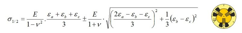
σ= material stress [N/mm2] ε= strain [m/m] Ε= modulus of elasticity, i.e. Young’s modulus [N/mm2] This version of Hooke's Law only applies to the uniaxial stress state. Biaxial and multiaxial stress states require extended versions. Note: In strain measurements, only, the difference between an initial output condition and a condition which occurs later can be determined. The initial condition may be a load-free condition, but it may also be a condition with significant pre-loading, for example due to the object's own weight as with a bridge. Preload or also residual stress conditions can only be measured if interference with the object is allowed e.g., making a small drill hole. The material stress σ should be calculated from the measured strain ε only, according to Hooke’s Law for the uniaxial stress state as in the equation stated above, if the strain ε is measured in the active direction of the force (0° direction). In the transverse direction (90° direction), there is no material stress present despite the measurable strain (transverse contraction, transverse dilation). Therefore, for reliable results the active direction of the force must be known and the strain must be measured in this direction. If this direction is unknown or only known approximately, then the measurements and their evaluation should be carried out with the biaxial stress state in unknown principal directions. In problems in experimental stress analysis, the uniaxial stress state is more the exception rather than the rule. The biaxial stress state is met far more often, and its determination should not be undertaken with the simple method used for the uniaxial stress state; this would lead to significant errors. For a plane stress condition, the extreme normal stresses σ1 and σ2 occur in the perpendicular directions 1 and 2. The stresses σ1 and σ2 are termed the principal stresses and similarly the directions 1 and 2 are the principal directions of the stress state. If the principal normal stresses and their active directions are known, the biaxial stress condition is unambiguously defined. Known principal directions of stress are found, for example, on the surface of a round cylindrical vessel under internal pressure, on a shaft loaded with pure torsion, and in an area away from the edges, on a bent plate. With other objects and with the simultaneous action of different variables, such as normal force and bending or torsion and bending, and so forth. the principal directions must be assumed to be unknown. The principal normal stresses σ1 and σ2 of the biaxial stress state are calculated according to the extended version of Hooke's Law from the measured principal strains ε1 and ε2, the material's modulus of elasticity E and Poisson's ratio v for the material: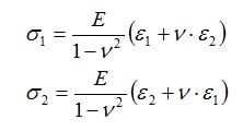 It is assumed that the stress σ3 in the principal direction 3 (perpendicular to the surface) is equal to zero.
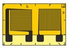
To simplify mounting procedures, X rosettes are suitable for measurements in the biaxial stress field with known principal directions. The axes of the two measuring grids must be mounted in alignment with the axes of the principal normal stresses (principal strain directions).
It is assumed that the stress σ3 in the principal direction 3 (perpendicular to the surface) is equal to zero.
To simplify mounting procedures, X rosettes are suitable for measurements in the biaxial stress field with known principal directions. The axes of the two measuring grids must be mounted in alignment with the axes of the principal normal stresses (principal strain directions).
 For objects of complex shape, with the superimposition of different types of loading (normal, bending or torsional loadings) or for points of inhomogeneity (e.g. changes in cross-sectional area), prediction of the principal directions of the stress state is generally not possible.
In each case where the directions of the principal stresses are not clearly defined, the stress analysis must be carried out according to the methods described below.
For objects of complex shape, with the superimposition of different types of loading (normal, bending or torsional loadings) or for points of inhomogeneity (e.g. changes in cross-sectional area), prediction of the principal directions of the stress state is generally not possible.
In each case where the directions of the principal stresses are not clearly defined, the stress analysis must be carried out according to the methods described below.
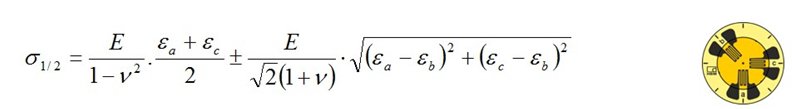
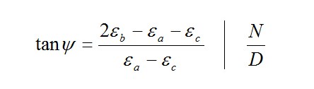 For the 0°/60°/120° rosette, according to the formula
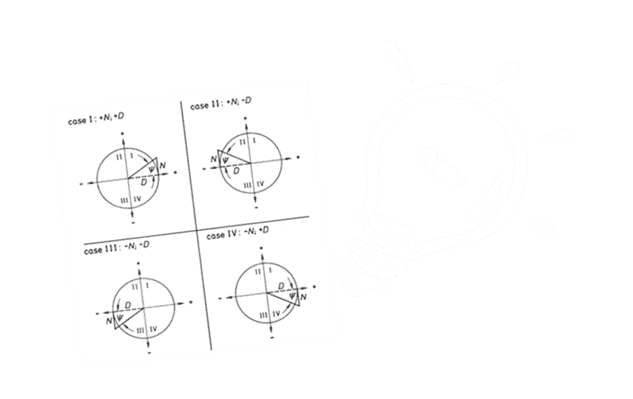
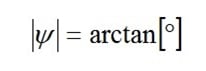
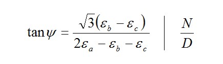 Note: The tangent of an angle in the right-angled triangle is the ratio of the opposite side (numerator N) to the adjacent side (denominator D):
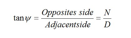 The figure below shows that the angle ψ may be in four different quadrants in the circular arc depending on the signs of the opposite and adjacent sides.
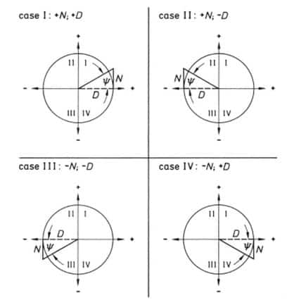
 Then the angle φ should be determined using the following scheme:
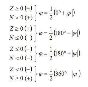 The angle φ found in this manner should be applied from the axis of the reference measuring grid a in the mathematically positive direction (counter-clockwise). The axis of the measuring grid a forms one arm of the angle φ. The other arm represents the first principal direction. This is the direction of the principal normal stress σ1 (identical with the principal strain direction ε1). The point of the angle is located at the intersection of the axes of the measuring grids. The second principal direction (direction of the principal normal stress σ2) has the angle φ +90°.

This will bring together HBM, Brüel & Kjær, nCode, ReliaSoft, and Discom brands, helping you innovate faster for a cleaner, healthier, and more productive world.
This will bring together HBM, Brüel & Kjær, nCode, ReliaSoft, and Discom brands, helping you innovate faster for a cleaner, healthier, and more productive world.
This will bring together HBM, Brüel & Kjær, nCode, ReliaSoft, and Discom brands, helping you innovate faster for a cleaner, healthier, and more productive world.
This will bring together HBM, Brüel & Kjær, nCode, ReliaSoft, and Discom brands, helping you innovate faster for a cleaner, healthier, and more productive world.
This will bring together HBM, Brüel & Kjær, nCode, ReliaSoft, and Discom brands, helping you innovate faster for a cleaner, healthier, and more productive world.