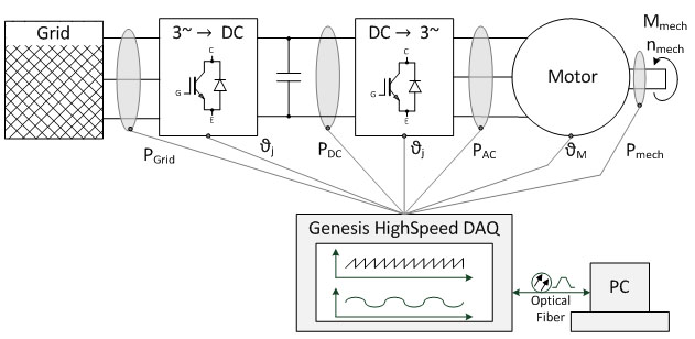
Various physical quantities must be recorded, saved and conditioned in measurements on energy-related systems, as shown in fig. 1.1 with a three-phase drive. Genesis HighSpeed data recorders enable synchronous acquisition of all important quantities in energy-related systems with a large number of channels and high sampling rates [1]. Especially in systems that are supplied with a three-phase current or generates a three-phasesystem, using space vectors to realize measured quantities makes for a clearer display that is easy to interpret. Space vectors can also be used to represent stationary operating states as well as dynamic balancing processes. In this paper, the defining equations for space vectors and rules for transformations to different coordinate systems will be explained first. Followed by an explanation of how to use space vectors to realize physical quantities of permanently excited synchronous machines (PSM). A Perception workbench has been prepared [3] to use when trying out these methods independently.
Calculation and Realization of Measured Quantities in Electrical Energy Technology as Space Vectors with HBM Perception Software
Summary
Space vectors are frequently used for clear and concise realization of measured quantities in electrical energy conversion systems such as transformers or induction motors. Additional information regarding the operating state of these energy converters can be determined if the time-dependent space vectors are realized as locus curves in the complex plane. To further simplify the representation of these measured quantities, the space vectors can be realized in rotating coordinate systems. This paper describes how to realize space vectors in different coordinate systems using the Perception software with an example based on a permanently excited synchronous machine.
1. Introduction
2. Space Vectors
K.P. Kovács developed the space vector theory in 1959 to facilitate a mathematical description of three-phase systems. It is often used to describe control methods for induction motors [4]. The electrical and magnetic quantities of a three-phase system can be mapped to a two-phase orthogonal system plus a zero-sequence system which is present under certain conditions. The two-phase orthogonal system can then be interpreted as a complex number which is designated as a space vector. The real and imaginary parts of the complex number correspond to the projections of the complex number displayed as a vector on the α and βaxes in the complex plan. Equation 1.01 defines the rules for calculating the complex space vectors ![]() from the three line variables x1, x2 and x3:
from the three line variables x1, x2 and x3:
![]()
α is a complex rotation operator. The corresponding zero-sequence system is calculated by
![]()
Fig. 2.1a shows the space vector ![]() in an orthogonal coordinate system.
in an orthogonal coordinate system.
The real part of the space vector appears on the abscissa α, the imaginary part on the ordinate β. In this figure the coordinate axes (α, β) are at rest. The line quantities can be obtained by projecting the space vectors onto the axes when rotated 120° a, b, c.
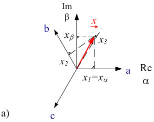
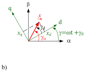
Fig. 2.1: Realization of space vectors in the complex plane a) in coordinate systems α, β at rest and b) in rotating coordinate systems
The Perception software offers predefined functions for transforming three-phase quantities (x1, x2, x3) into space vector quantities:
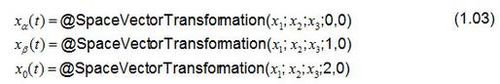
Perception also provides a mathematical function for the reverse transformation, to calculate the corresponding line quantities from space vector quantities:
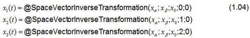
The meanings of the various transfer parameters are described clearly online in the Help section, available when the formulas are entered in Perception.
Using these transformation functions, calculations can now be performed in the space vector domain. Then the results of the calculations can be displayed again as line quantities.
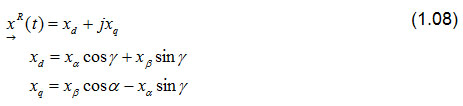
The computing overhead can be reduced for many applications while improving the clarity of results obtained, if the space vectors are realized in rotating coordinate systems. Until now, we have examined coordinate systems with the α and β axes at rest. Now, we will also consider space vectors in a d,q coordinate system which is rotated by any time-dependent angle γ(t) in comparison to the original α,β coordinate system. Derivation of the transformation rules is simplified, if the space vectors are described in polar display. The space vector in the coordinate system at rest in polar display is notated as follows:
![]()
As shown in fig. 1.1b), this space vector can also be described in a rotating coordinate system with d and q axes. The superscriptR indicates that the space vector is represented in rotating coordinate systems. In polar display the amount does not change in different coordinate systems. Only the angle has to be adjusted.
![]()
Space vectors are transformed from one coordinate system to another by multiplying them by the rotation operator ejγ.
![]()
Euler's formula ejγ = cos(γ)+j sin(γ)can be used to calculatethe components of the rotating space vector.
Perception provides the following functions to transform the three line quantities x1, x2and x3 into a rotating space vector.
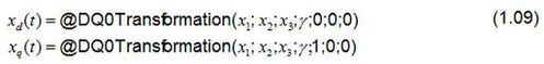
The angle γrequired for the transformation is either calculated or read by a position encoder, depending on the application.
3. Permanently Excited Synchronous Machine
Use of space vectors in different coordinates will be explained basedon the example of a permanently excited synchronous machine [4]. To keep the description of the machine simple, an isotropic synchronous machine will be considered. This means the magnetic field can expand in the machine independently of direction. Fig. 3.1a) shows a surface-mounted, permanent-magnet synchronous motor (PMSM). This type of machine may be considered to be approximately isotropic. The number of pole pairs in the machine shown here is p=2. To obtain a widely usable description of the machines, the actual machines are described with models, with p=1 as the number of pole pairs. The simple space vector model of the PSM in fig. 3.1b) will serve to extend the description. To do this we must take into consideration the correlation between the mechanical speed n and the electrical frequency f where are:
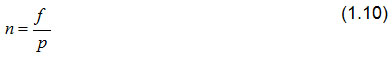
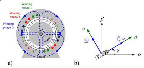
Fig. 3.1: a) Basic layout of a PSM b) space vector model of a PSM.
If a position encoder is placed on the shaft of the synchronous machine, the number of polar pairs p and an offset angle γ0 of the angle γ required for the space vector transformation can be calculated. The function
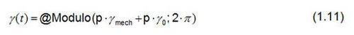
is defined in Perception and used for this purpose. The offset angle γ0 takes into consideration the mechanical offset between the north pole of the rotor and the zero position of the position encoder.
A no-load test is used to determine the offset angle γ0. To do this, the synchronous machine is driven mechanically by the shaft. Fig. 3.2 shows the star voltage u1as a function of time and the mechanical angle γmechread by the position encoder. The offset angle γ0 can be read from the time offset between the zero crossing with negative slope of the voltage u1 and the zero position of the position encoder.
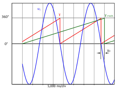
Fig. 3.2: Time-dependent curve of the star voltage u1, mechanical angle γmech and electrical angle γ
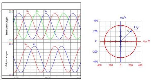
The star voltages induced in the no-load test are shown in fig. 3.3. These three sinusoidal voltages form a symmetrical three-phase system if the amplitudes of the voltages are equal in magnitude and the phase offset between the voltages is 120°. The space vector components (uα,uβ) belonging to this three-phase voltage are also shown in fig. 3.3a) as a function of time. Given a symmetrical voltage system, a phase shift of 90° is established between the space vector components (uα,uβ).
If the space vector components are represented in an xy plot, the peak of the voltage space vector describes a circle, as shown in fig. 3.3b). If the trajectory of the curve deviates from an ideal circle, it can be seen at a glance that the three voltages do not form a symmetrical three-phase system.
 b)
b)
Fig. 3.3: Time-dependent curve of star voltages u1,u2 and u3 of the space vector components uα,uβ (a). Trajectory of the voltage space vector (b)
Now if the voltage space vector components uα and uβ are displayed in a rotating coordinate system with components ud and uq, these quantities which vary over time, become constant quantities. Components ud and uq of a symmetrical three-phase system are shown in fig. 3.4, once as a function of time and once in the complex plane. Asymmetrical three-phase system is represented in the complex plane as a pointer at rest with a constant length.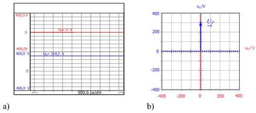
Fig. 3.4: Time-dependent curve a) of the voltage space vector components ud and uq and
b) of the voltage space vector in the rotating coordinate system.
Summary
This report presents signal conditioning with a Genesis HighSpeed data recorder and the Perception software using space vector calculations. The transformation rules were described for calculating the space vectors in different coordinate systems from the raw data of a Genesis HighSpeed data recorder. The coordinate systems were presented and explained based on the example of a no-load test with a synchronous machine using different display methods for the space vectors with Perception. For further practical testing, of the calculation methods with space vectors in energy technology, HBM provides a workbench running under Perception [3].
Bibliography
[1] D. Eberlein; K. Lang; J. Teigelkötter; K. Kowalski: Elektromobilität auf der Überholspur: Effizienzsteigerung für den Antrieb der Zukunft [Electromobility in the fast lane: increased efficiency for the drive of the future]; proceedings of the 3rd conference of Innovation Messtechnik [Innovation in Measurement Technology]; May 14, 2013
[2] Berechnung von Leistungsgrößen mit Perception-Software
[Calculating power values with Perception software] https://www.hbm.com/de/3783/berechnung-von-leistungsgroessen-mit-perception-software/
[3] www.hbm.com
[4] J. Teigelkötter: Energieeffiziente elektrische Antriebe [Energy-efficient electric drives], 1st edition, Springer Vieweg Verlag, 2013; ISBN 3-8348-1938-3